
Structural mechanics
Stresses, strains, reactions and safety factor for parts, framed structures and shells, from linear to nonlinear.
- 2D, axisymmetric and 3D solids
- Trusses, frames, beams
- Shells
- Modal and buckling
- Plasticity
- Hyperelasticity
- Contact
Build the geometry, generate the mesh, choose the physics and solve: structures, heat, fluids and electromagnetics, on their own or coupled. Every calculation runs on your own computer, with nothing to install, and you can watch the convergence live.
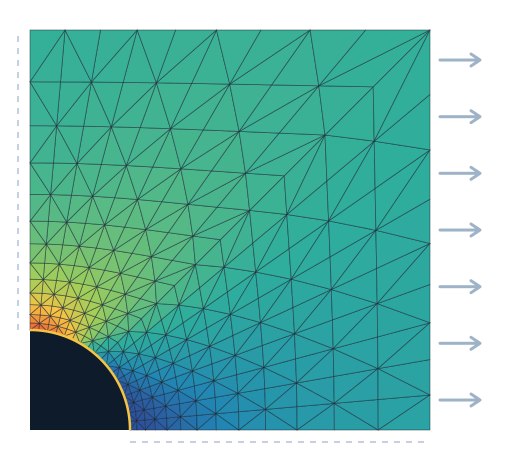
Combine whatever physics your problem calls for. The coupled-physics engine solves the fields in a single system, using Newton's method, on triangles, tetrahedra or hexahedra.
Stresses, strains, reactions and safety factor for parts, framed structures and shells, from linear to nonlinear.
Temperature and heat flux at steady state or over time, with a timeline and animation.
Velocity, pressure, flow rates and wall forces, with arrows and streamlines, in 2D and 3D.
Potential, electric field, current density and magnetic field, with the generated heat passed on to the thermal analysis.
Fully coupled in a single system of equations, or sequential when that is enough. Moving mesh (ALE) for fluid-structure interaction.
From steady-state to frequency response, with plots, click-to-probe, contour lines, deformed shape and export.
Numbered steps, in the order the problem is built, and a guide that shows the next step and does it in one click. The project tree keeps everything and can be edited at any time.
Parametric 2D and 3D shapes with Boolean operations, or imported DXF and STL files.
Materials from the library, click-to-apply boundary conditions and loads written as expressions.
Delaunay triangulation with a size field; hexahedra and tetrahedra in 3D.
Direct and iterative solvers selected automatically (or by AI, if you like), running in Web Workers, with WebGPU when available and a live convergence plot.
Color maps, deformed shape, arrows, streamlines, probes, plots and CSV.
The server is optional: it only stores models and, if you choose, computes large tetrahedral meshes and STEP files in a separate worker.
The interface never waits for the solver: meshing, assembly and solving run in Web Workers, and each physics module is downloaded only when the model needs it.
Time per stage in the browser · 4 cores, no GPU

Engineering on Web CAD is our free parametric CAD in the browser: constrained sketches, parts, assemblies and technical drawings. Export the part as STL, which Engineering on Web FEA opens directly in the browser, or as STEP, which the server worker turns into a tetrahedral mesh.
No. Engineering on Web FEA runs in your browser (a recent version of Chrome, Edge, Firefox or Safari). Meshing, matrix assembly and the solvers run in Web Workers on your own computer; the server only stores models and, if you choose, computes large meshes.
Each physics is added to the program only after passing benchmark cases with known solutions, such as the Timoshenko beam, the plate with a hole, the Lamé cylinder, the Ghia lid-driven cavity and the Scordelis-Lo roof. Even so, always check the mesh and boundary conditions of your model.
Structural mechanics (2D, axisymmetric and 3D solids, trusses, frames, beams and shells, modal, buckling, plasticity, hyperelasticity and contact), heat transfer (conduction, convection and radiation, steady-state and transient), fluids (laminar, turbulent, two-phase, Brinkman and Darcy), electromagnetics and the couplings between them, such as thermal-structural, Joule heating and fluid-structure interaction.
It is optional and off by default. When enabled, before each run the AI (via Puter.js) receives a summary of the model and the run times already measured on your machine, and chooses the solver strategy: direct or iterative, GPU usage, Newton damping, pseudo-time stepping. It never touches tolerances, mesh or physics, so the result has the same accuracy; if a suggestion fails, the run is repeated with the original settings.
No. When WebGPU is available, the conjugate gradient runs on the GPU in mixed precision; without it, or if the GPU cannot reach the requested tolerance, the calculation automatically falls back to the CPU. The GPU is an accelerator, never the source of truth.
It depends on your machine. As a reference, a 2D beam with 49,302 degrees of freedom solves in 7.2 s on a 4-core computer without a GPU. For very large models, gmsh tetrahedral meshing and STEP files, an optional server-side worker is available.
It imports DXF for 2D geometry and STL for 3D in the browser; STEP goes through the server worker. It exports the model as JSON, the nodal table as CSV, the image as PNG and, via the server, VTU for ParaView.
Open one of the ready-made examples and solve it in seconds, right in your browser.
Open the simulator